Anytime-Valid Regression Adjusted Causal Inference

Investigating the methods described in Anytime-Valid Linear Models and Regression Adjusted Causal Inference in Randomized Experiments by Lindon, et al. via simulations.

Randomized experiments (A/B tests) are ubiquitous in both academia and the tech sector. They enable robust causal inference regarding the impact of interventions on user or participant outcomes. Under randomization, various estimators provide valid estimates of the average treatment effect (ATE), defined as \(\tau = E[Y_i(1) - Y_i(0)].\) These estimators typically yield both point estimates and confidence intervals (CIs) such that \[P(\tau \in \text{CI}) <= \alpha,\] where \(\alpha\) is the significance level and \(\text{CI}\) is a random interval constructed from our data.

One major issue with common estimators like ordinary least squares (OLS) is that the statistical guarantees for their confidence intervals only hold for a pre-specified sample size \(N\). A surprisingly common practice is to collect some data, estimate \(\tau\) and its corresponding 95% CI, and then, if the effect is large but not statistically significant, collect more data and re-estimate \(\tau\). This process of “data-peeking” may be repeated multiple times. However, such practices violate the statistical guarantees of standard confidence intervals, causing the probability of a Type I error to far exceed the nominal significance level \(\alpha\).

To address this issue, researchers at Netflix have developed anytime-valid Confidence Sequences (CSs) for linear regression parameters. These CSs have the property that \[P(\forall n, \delta \in \text{CS}_{\delta, n}) \geq 1 - \alpha,\] where \(\delta\) represents the regression parameter. Essentially, this means that you can estimate the parameter and update the CS as often as you like, and the probability of committing a Type I error will always remain below \(\alpha\).

This method is not only practically significant but also easy to implement using standard linear regression outputs in R. The simulations that follow will demonstrate the usefulness of this approach.

Simulate RCT

These simulations will rely on the following packages:

Dependencies

library(dplyr)
library(ggplot2)

Data generation and helper functions

We simulate a simple randomized controlled trial (RCT) where binary treatment is assigned randomly. The potential outcomes are defined by \[Y_i(W_i) = 0.5 + 0.5*W_i + 2*X_{i1} + 1.2*X_{i2} + 0.4*X_{i3} + \epsilon_i\]

where \(W_i\)​ indicates the treatment status of unit \(i\), the true average treatment effect (ATE) is \(\tau = 0.5\), and \(\epsilon_i \sim \text{Normal}(0, 1)\).

In this setting, a simple regression of \(Y_i\)​ on an intercept and \(W_i\)​, i.e. \(Y_i \sim \alpha + \tau * W_i\)​, is equivalent to the difference-in-means estimator and produces an unbiased estimate \(\hat{\tau}_{DM}\) of \(\tau\). Similarly, a covariate-adjusted regression, given by \(Y_i \sim \alpha + \tau * W_i + \beta^T*X_i\), also provides an unbiased estimate \(\hat{\tau}_{CA}\), but with lower variance than \(\hat{\tau}_{DM}\).

First, we define a function to simulate a random tuple \((X_i, W_i, Y_i)\) according to the RCT setup described above:

draw <- function(arm, ate, sigma = 1.0) {
  covar_coef <- c(2, 1.2, 0.4)
  covar <- rbinom(3, size = 1, prob = c(0.1, 0.5, 0.9))
  y <- 0.5 + ate*arm + drop(covar_coef %*% covar) + rnorm(1, 0, sigma)
  cbind(data.frame("y" = y, "t" = arm), data.frame(t(covar)))
}

Next, for a dataset comprising these units \(\{(X_i, W_i, Y_i)\}_{i=1}^N\)​, we construct a function to estimate both \(\hat{\tau}_{DM}\) and \(\hat{\tau}_{CA}\)​, along with their corresponding exact and asymptotic confidence sequences (CSs):

compare <- function(model_ca, model_dm, data, iter, ate = 0.5) {
  seq_f <- sequential_f_cs(model_ca, phi = 10)
  seq_f_dm <- sequential_f_cs(model_dm, phi = 10)
  seq_asymp <- ate_cs_asymp(model_ca, treat_name = "t", lambda = 100)
  seq_asymp_dm <- ate_cs_asymp(
    model_dm,
    lambda = 100,
    treat_name = "t"
  )
  comparison_df <- data.frame(
    "i" = iter,
    "method" = c(
      "f_test",
      "f_test_unadj",
      "asymp",
      "asymp_unadj"
    ),
    "estimate" = c(
      subset(seq_f, covariate == "t")$estimate,
      subset(seq_f_dm, covariate == "t")$estimate,
      seq_asymp$estimate,
      seq_asymp_dm$estimate
    ),
    "lower" = c(
      subset(seq_f, covariate == "t")$cs_lower,
      subset(seq_f_dm, covariate == "t")$cs_lower,
      seq_asymp$cs_lower,
      seq_asymp_dm$cs_lower
    ),
    "upper" = c(
      subset(seq_f, covariate == "t")$cs_upper,
      subset(seq_f_dm, covariate == "t")$cs_upper,
      seq_asymp$cs_upper,
      seq_asymp_dm$cs_upper
    )
  )
  comparison_df$covered <- (
    comparison_df$lower <= ate & ate <= comparison_df$upper
  )
  return(comparison_df)
}

Finally, we create a function that simulates an experiment of size \(N\) where each tuple \((X_i, W_i, Y_i)\) is received sequentially. At each sample size \(n \leq N\), we re-estimate \(\hat{\tau}_{DM}\), \(\hat{\tau}_{CA}\)​, and their CSs:

simulate <- function(model_ca_fn, model_dm_fn, draw_fn, n, ate) {
  # Warm-start with 20 observations so that no regression coefs are NA
  # at any point
  df <- do.call(rbind, lapply(1:20, function(x) draw_fn(ate)))
  estimates <- data.frame()
  for (i in 1:n) {
    observation <- draw_fn(ate)
    df <- rbind(df, observation)
    model <- model_ca_fn(df)
    model_dm <- model_dm_fn(df)
    estimates <- rbind(
      estimates,
      compare(model, model_dm, df, iter = i, ate = ate)
    )
  }
  estimates <- estimates |> 
    mutate(
      stat_sig = 0 < lower | 0 > upper,
      method = case_when(
        method == "asymp" ~ "Sequential asymptotic CS",
        method == "asymp_unadj" ~ "Sequential asymptotic CS w/o covariates",
        method == "f_test" ~ "Sequential CS",
        method == "f_test_unadj" ~ "Sequential CS w/o covariates",
        method == "lm" ~ "Fixed-N CS",
        method == "lm_unadj" ~ "Fixed-N CS w/o covariates"
      )
    ) |>
    group_by(method) |>
    mutate(transition = (!lag(stat_sig, default = FALSE)) & stat_sig) |>
    mutate(
      stat_sig_i_min = if_else(
        any(stat_sig & !lag(stat_sig, default = FALSE)),
        min(i[stat_sig & !lag(stat_sig, default = FALSE)]),
        NA_integer_
      ),
      stat_sig_i_max = if_else(
        any(transition),
        max(i[transition]),
        NA_integer_
      )  
    ) |>
    ungroup()
  return(estimates)
}

Run the simulation

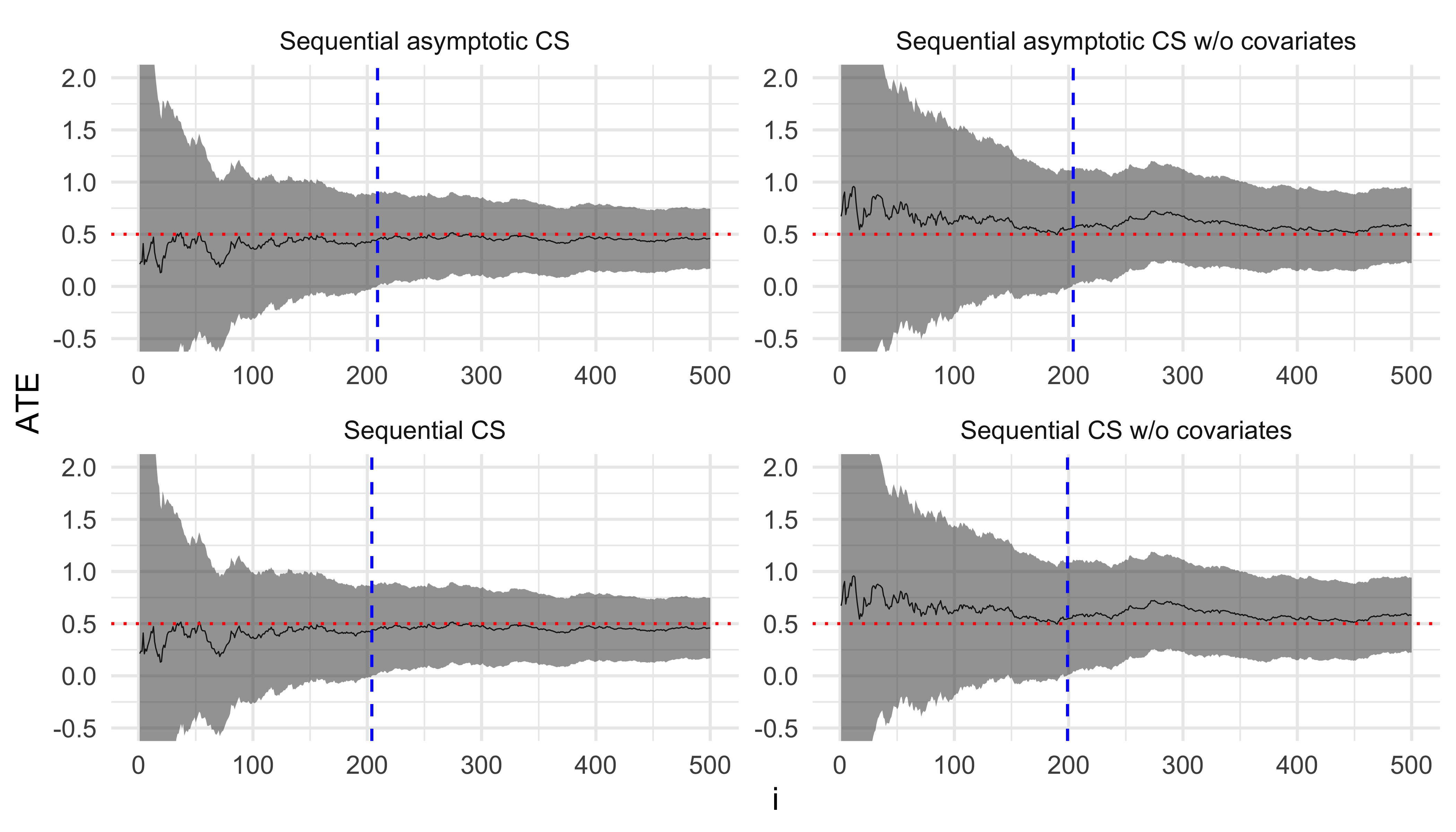
We then run our simulation for \(N = 500\) and plot the estimates \(\hat{\tau}_{DM}\) and \(\hat{\tau}_{CA}\)​ along with their CSs at each step. The red dotted line is the true value of \(\tau\) and the vertical blue line indicates the sample size when the corresponding estimator becomes statistically significant.

estimates <- simulate(
  model_ca_fn = function(data) lm(y ~ ., data),
  model_dm_fn = function(data) lm(y ~ t, data),
  draw_fn = function(ate) draw(rbinom(1, 1, 0.5), ate = ate),
  n = 500,
  ate = 0.5
)

ggplot(estimates, aes(x = i, y = estimate, ymin = lower, ymax = upper)) +
  geom_line(linewidth = 0.2) +
  geom_ribbon(alpha = 0.5) +
  geom_hline(yintercept = 0.5, linetype = "dotted", color = "red") +
  geom_vline(aes(xintercept = stat_sig_i_max), linetype = "dashed", color = "blue") +
  facet_wrap(
    ~ method,
    ncol = 2,
    scales = "free",
  ) +
  coord_cartesian(ylim = c(-0.5, 2)) +
  labs(y = "ATE") +
  theme_minimal()

Simulate non-fixed-probability randomized data (but known propensity scores)

Next, we simulate a randomized experiment where propensity scores are generated as a known function of covariates. Specifically, the propensity score for unit \(i\) is given by \[e_i = 0.05 + 0.5*Z_{i1} + 0.3*Z_{i2} + 0.1*Z_{i3},\]​ where \(\{Z_{i1}, Z_{i2}, Z_{i3}\}\) are binary covariates. The potential outcomes are defined as \[Y_i(W_i) = 0.5 + 0.5*W_i + 3*X_{i1} + 3*X_{i2} + 1*X_{i3} + 0.5*Z_{i1} + 0.3*Z_{i2} + 0.1*Z_{i3} + \epsilon_i,\] with \(W_i\)​ representing the treatment status, the true average treatment effect (ATE) \(\tau = 0.5\), and \(\epsilon_i \sim \text{Normal}(0, 1)\). In this setup, a simple regression of \(Y_i\)​ on an intercept and \(W_i\), weighted by the inverse propensity scores \(\frac{1}{e_i}\), yields an unbiased estimate \(\hat{\tau}_{IPW}\)​ of \(\tau\). Similarly, the covariate-adjusted regression \(Y_i \sim \alpha + \tau * W_i + \beta^T*X_i\), when weighted by the inverse propensity scores, produces an unbiased estimate \(\hat{\tau}_{CAIPW}\) that typically has lower variance.

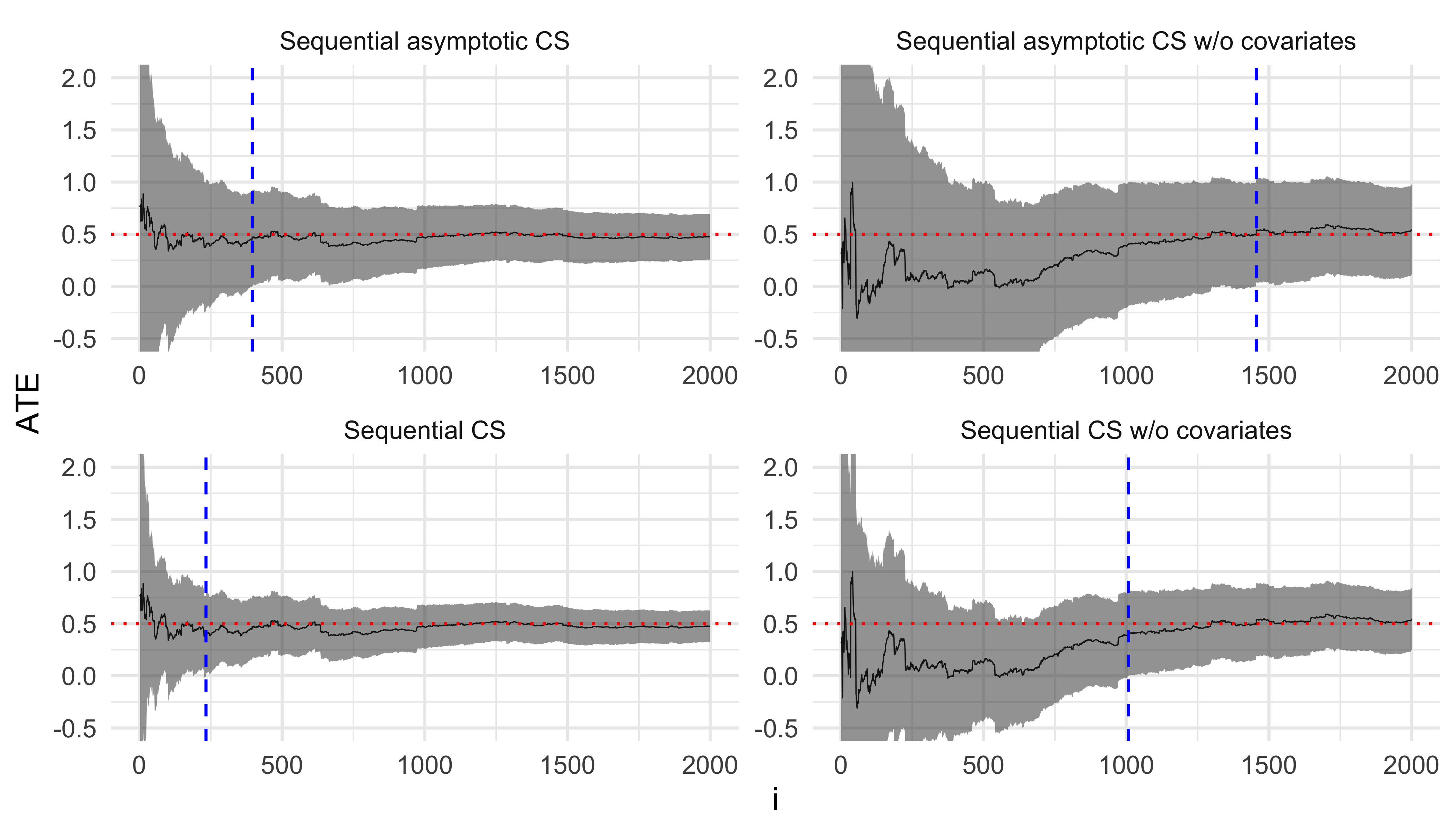
We then create a function to generate data based on this experimental setup and run our simulation for \(N = 2000\). As before, we plot \(\hat{\tau}_{IPW}\), \(\hat{\tau}_{CAIPW}\) and their corresponding confidence sequences (CSs) at each step.

draw_prop <- function(ate = 2.0, sigma = 1.0) {
  prop_covar_coef <- c(0.5, 0.3, 0.1)
  prop_covar <- rbinom(3, size = 1, prob = c(0.1, 0.4, 0.7))
  prop <- drop(prop_covar_coef %*% prop_covar) + 0.05
  covar_coef <- c(3, 2, 1)
  covar <- rbinom(3, size = 1, prob = c(0.25, 0.5, 0.75))
  arm <- rbinom(1, 1, prop)
  y <- (
    0.5
    + ate*arm
    + drop(covar_coef %*% covar)
    + drop(prop_covar_coef %*% prop_covar)
    + rnorm(1, 0, sigma)
  )
  cbind(data.frame("y" = y, "t" = arm, "p" = ifelse(arm, prop, 1 - prop)), data.frame(t(covar)))
}

# Simulation estimates
estimates <- simulate(
  function(data) lm(y ~ . - p, data, weights = 1/data$p),
  function(data) lm(y ~ t, data, weights = 1/data$p),
  draw_fn = function(ate) draw_prop(ate = ate),
  n = 2000,
  ate = 0.5
)

ggplot(
  estimates,
  aes(x = i, y = estimate, ymin = lower, ymax = upper)
) +
  geom_line(linewidth = 0.2) +
  geom_ribbon(alpha = 0.5) +
  geom_hline(yintercept = 0.5, linetype = "dotted", color = "red") +
  geom_vline(aes(xintercept = stat_sig_i_max), linetype = "dashed", color = "blue") +
  facet_wrap(
    ~ method,
    ncol = 2,
    scales = "free",
  ) +
  coord_cartesian(ylim = c(-0.5, 2)) +
  labs(y = "ATE") +
  theme_minimal()

As expected, including covariates significantly improves the precision of our ATE estimates.

Type 1 error control

Finally, we assess the empirical Type I error control by running multiple simulations under the null hypothesis (i.e., with \(\tau = 0\)). For each simulation, we record whether a Type 1 error is ever committed; that is, whether the CS ever fails to cover \(\tau\). The overall empirical Type I error is then the fraction of simulations in which the CS commits a Type I error. This global guarantee is analogous to the property of a standard CI: before data is observed, we know that the probability of a Type I error is \(\leq \alpha\).

estimates <- lapply(
  1:100,
  function(index) {
    simulate(
      model_ca_fn = function(data) lm(y ~ ., data),
      model_dm_fn = function(data) lm(y ~ t, data),
      draw_fn = function(ate) draw(rbinom(1, 1, 0.5), ate = ate),
      n = 1000,
      ate = 0
    ) |>
    mutate(sim_i = index)
  }
)

error_rate <- estimates |>
  bind_rows() |>
  group_by(sim_i, method) |>
  summarize(any_error = !all(covered)) |>
  ungroup() |>
  group_by(Method = method) |>
  summarize(`Type 1 error` = mean(any_error))

error_rate

# A tibble: 4 × 2
  Method                                  `Type 1 error`
  <chr>                                            <dbl>
1 Sequential CS                                     0.04
2 Sequential CS w/o covariates                      0.04
3 Sequential asymptotic CS                          0.04
4 Sequential asymptotic CS w/o covariates           0.03

We see that, indeed, Type 1 error is \(\leq \alpha = 0.05\) for all estimators.

Credits

A lot of the code for this was based on the paper’s official repository and was crafted in tandem with my trusty AI assistant (ChatGPT).